
The site is characterized by complex structure, with high velocity contrasts between individual blocks, (vS = 2600 m/s)/( vS = 425 m/s); also the vP/vS velocity ratio is up to 5. Numeric instabilities have been found at contacts between blocks with high and low vP/vS ratios. A simple trick to stabilize the calculations for long FD runs (e.g. 20 000 time levels, or more) has been suggested. It consists of a special algorithmic treatment of the material discontinuities, preventing mixing of very large and very small values of the so-called effective material parameters within a grid cell. Appendix provides a comparison of the present FD method with an independent method for a model with non-planar topography and several vP/vS ratios.
Figure 1: The computational model. (a) The model constitution of blocks (see Table 1). (b-c) Details of the upper part of the model. The arrows point at the contacts of the blocks that produced instabilities.
| block No. | 1 | 2 | 3 | 4 | 5 |
| vP | 460 | 1500 | 1800 | 2600 | 4200 |
| vS | 230 | 300 | 425 | 700 | 2600 |
| r | 1750 | 2000 | 2200 | 2300 | 2600 |
| Q | 20 | 30 | 40 | 60 | 200 |
It is a 2D model with flat surface topography (see Fig. 1 and Table 1 ). The sedimentary valley structure consists of blocks with constant velocities (vP and vS), densities (r), and quality factors (QP and QS). Our model is purely linear. The intention is to simulate the response of the valley with respect to the plane wave vertically incident from below.
The simulation is performed for P-SV case. It is based on FD method using the PS2 scheme (Zahradník, 1995) with some modifications described below. The PS2 is a scheme in displacement components, 2nd order accurate inside the medium, employing heterogeneous formulation of the elastodynamic equation on a regular square grid. The free surface is treated by vacuum formalism with 1st order accuracy. The attenuation, described for simplicity by QP=QS, proportional to frequency, is included in the equations of motion by a term proportional to velocity. The quality factor is spatially variable. The prescribed Q values are assumed to be valid at 2Hz. The modeling consists of two steps, A and B. Step A is calculation of the pseudoimpulse response (PIR) with respect to the vertically incident plane wave excitation, whose time history is a Ricker wavelet of a short duration, tp = 0.25 seconds. Step B is calculation of the response with respect to the prescribed excitation represented by an earthquake record. Only step A is presented in this paper.
Numerical parameters of our modeling are summarized in Table 2.
| dx = dz | dt | fac | Nx | Nz | Nt |
| 5.0 | 0.0007 | 4.6 | 1350 | 150 | 21500 |
The simulation of the pseudoimpulse response 15 seconds long took about 750 minutes on HP 735/125 workstation.
 Figure
2: The effective parameters (m)ef
(dashed-dotted), (l)ef (thin
solid), (l+2m)ef
(thick soid) computed correctly by geometric averaging of each of these
three values separately. The dashed thick and thin lines show the value
of (l+2m)ef
and (l)ef indirectly computed
from the known effective parameters (m)ef,
(l)ef and/or (l+2m)ef
respectively.
Our code represents the model by polygonal blocks. Neither nodes of the blocks, nor their sides coincide with gridlines, in general, thus automatically computed effective material parameters may vary along the block boundaries in a complex way, see Fig. 1a (e.g., see the interface between blocks 2 and 3, or 3 and 4). In a very early stage of this work a numerical instability of the P-SV simulation was found, that could not be removed by any decrease of the steps dx, dt. (While SH case for the same model was completely free of any instability.) The problem was spatially localized to the edges of the basin; see details marked in Figs. 1b,c. As reported in Zahradník (1995), the PS2 scheme requires that gently sloping interfaces outcropping at the surface are locally transformed into short vertical segments coinciding with a grid line. We used this trick in the model of Fig. 1, too, but it only postponed the catastrophic instability by tens of timelevels (i.e. by 0.01 s).
The effective parameters (EPR), that represent a key feature of the PS2 method, are geometric averages of the true elastic parameters along so-called grid legs between two neighbouring grid lines. In our code, two sets of EPR are directly calculated: (l+2m)ef, and (m)ef. The term "directly" means calculation after definition formulas, e.g. equation (2) of Zahradnik (1995). Then, using these two, the effective l is indirectly calculated as (l+2m)ef- 2(m)ef. This, of course, is not the same as the directly calculated (l)ef. We hypothetized that the mentioned instabilities could be just of this reason. Therefore, in an auxiliary code, we directly calculated all the three: (l+2m)ef, (l)ef, (m)ef. These parameters have been compared in Fig. 2 for two velocity values. Taking the direct calculation of all the three EPR as a reference, the error in evaluating (l)ef may be greater than 200%, for high contrasts of m (1:10). (Let us stress that this contrast in m doesn't necessarily mean contrast in vS between the neighbouring blocks as the density also plays a role.) This explains why the EPR calculated in our main code (that one using direct EPR for l+2m and m, but indirect one for l) display some 'overshoots' marked by the narrow bright spots along certain boundaries; see a detail of the model l values in Fig. 3.
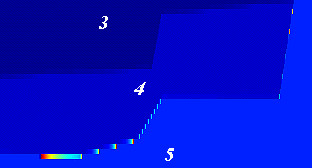 Figure
3: Detail of the lower-right part of the basin - the model parameter (l)ef
affected by the incorrect indirect computation (see Fig.
2). The 'overshoots' are visible as the narrow bright spots along certain
boundaries (between blocks 4 and 5 depicted in Fig.
1). Shown is the vertical parameter, corresponding to A in Fig.
4.
However, in spite of the fact that the FD code was modified so as to all the three effective parameters (l+2m)ef, (l)ef, (m)ef were calculated directly, the instabilities mentioned above were not removed.
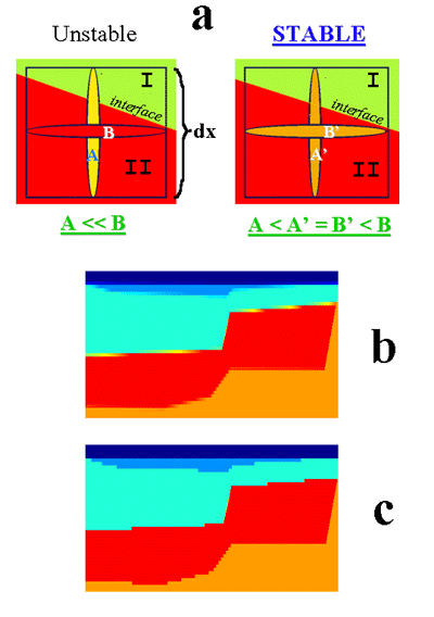 Figure
4: The model parameters treatment for stabilization purposes. (a) Shows
that in case of contrast of parameters in blocks I and II,
and when the effective parameters are A <<
B, we substitute A®
A' and B® B',
while A < A' º
B' < B. (b,c) Are
details of the model for vertical (b) and horizontal (c) parameters along
the slightly dipping interface between two blocks. After the stabilization
trick, the new effective parameters ale looking like in (c) for both vertical
and horizontal parameters ((a) right).
Therefore, the following stabilization approach was adopted (see also Fig. 4a): As an example, let A and B are EPR values very different from one another. The large difference between A and B comes from the geometrical averaging of two contrasting media parameters (A value), while B is equal to parameter value of block under the interface, see Fig. 4a. The stabilization trick is as follows: For A << B, we substitute A® A' and B® B', while A < A' º B' < B. For example (A = 1·109 Pa,B = 9·109 Pa)®A' = B' = 5·109 Pa. The other parameters in the gridcell are treated in the same way as in the "full-form" formulas of Zahradník (1995). This trick is equivalent to surrounding the blocks with one-gridstep thick belt of varying parameters whose values are still in the range given by the parameters of the neighbouring blocks, see Figs. 4b,c. This creates a 1-gridcell-thick block with varying parameters supplying the original interface without bluring it, compare Figs. 4b and 4c. The same stabilization process is sometimes also needed in other cases (e.g. in the random medium, Oprsal & Zahradník, 1997).
It is interesting to note that many other stabilization tricks (several dozens of experiments !) were attempted with absolutely no success. For example, we artificially substituted velocities in the upper left and right parts of block 4 with parameters of block 2 and/or 3 (Fig. 1) in order to decrease the vP/vS velocity contrast, etc. Compared to these trials, an appreciable fact is that the successful stabilization introduced above allowed calculations with the very high vP, vS contrasts, as well as very high vP/vS ratio contrasts, prescribed in the original model (Fig. 1, Table 1), without any necessity to change these values in the whole blocks.
Although a minor modification of the interfaces is (locally) introduced by the stabilization, the traction continuity is not violated (Oprsal & Zahradník, 1999). Thus the overall effect of the curved material discontinuities is modelled satisfactorily. To show this, at least for a particular model, we have tested the method at the most contrasting discontinuity, i.e. the non-planar free surface, by comparison with the finite-element method; see appendix.
 Figure
5: The horizontal component of the pseudoimpulse response for the Volvi
Lake with respect to a vertically incident plane S wave for the P-SV
case. It is accurate up to 4.6 Hz.
The notable features are as follows: a) the edge effects, including fast spatial changes of the wavefield, as well as the edge-generated surface waves, b) large durations inside the valley (dependent, of course, on the adopted attenuation model), c) combined effects of the deep valley structure and the localized shallow layers, and d) the mode conversion.
As seen from the result in Fig. 5, the surface motions vary significantly along the valley as regards their peak values, spectral content and durations. This important conclusion has been obtained in spite of the fact that the excitation was only a simple plane wave.
More results, plus those presented here, are available in a numerical form (as ASCII files) on the WWW (or see Web site 1).
 Figure
A1: The ridge model (Gaffet and Bouchon, 1989). Receivers R1..R19
depicted by crosses, located on a free surface with a constant horizontal
spacing of 166.66 m, R1 is on the top of the ridge (h = 375
m); R14 .. R19 are located in depth of z = 615.6 m
(R15 is not displayed), the horizontal distance of these receivers
is as follows: R14 = 0.0 m, R15 = 11.165 m, R16 =
166.667 m, R17 = 333.333 m, R18 = 500.0 m, R19 = 1000.0
m.
The source is a vertical force applied at the base, in the centre of the hill, its time function is defined as: f(t) = (b-0.5)exp(-b), b = [p(t-ts)/tp]2, with tp = 0.4875s, ts = 0.4875 s . The time window was t Î (0s,4.0s) The surface shape is (Gaffet and Bouchon, 1989): s(x) = h(1.0-a)exp(-3a), a = (x/l)2, with h = 375 m, l = 1000 m, where h and l denote the height and the half-width of the hill; x Î (0,l), while s(x) = 0 for x > l.
Receivers R1 .. R13 are located on a free surface with a constant horizontal spacing of 166.66 m, the R1 receiver is on the top of the ridge (see Fig. A1). Receivers R14 .. R19 are located in depth z = 615.6 m, the horizontal distance of these receivers is as follows: R14 = 0.0 m, R15 = 11.165 m, R16 = 166.667 m, R17 = 333.333 m, R18 = 500.0 m, R19 = 1000.0 m. There are no artificial reflections arriving to any of the receivers during the defined time window. Computation was done for a series of cases with vP = 2000 m/s and vS = 1400 , 1000 , 750 , 500 , 300 , 200 , 0.01 m/s (the last one being just formal).
The results (vertical component) are presented for two cases: vS = 0.01 m/s, and vS = 500 m/s (vP/vS = 4) in Fig. A2. The good agreement visible in these two cases was also found in all trials with vS ³ 500 m/s, while the two models with vS = 300 and, 200 m/s had worse agreement between FD and FEFD synthetics in receivers R15..R19.
 Figure
A2: The comparison between the method of the present paper, and FDFE
hybrid method of Moczo et al. (1997) for the ridge model described in Fig.
A1.
Because the 'liquid ridge' case with the formal value of vS = 0.01 m/s does not suffer of this disagreement, it is probable that the differences come from different behaviour of the methods in treating the surface computations for high vP/vS ratios, larger than 4.
The comparison in GIF and EPS formats for other vP/vS ratios is available at WWW (or see Web site 2).
This work was performed within the EU sponsored Inco-Copernicus ISMOD
project, based on the EURO-
SEISTEST data. Additional support was provided from the Inco-Copernicus
COME project, the Grant Agency of the Czech Republic GA CR 205/1743, the
Charles University Grant 5/97, and the Czech Ministry of Education, Youth
and Sports, grants No OK 278, ME 060. The authors thank M. Pakzad who participated
in the numerical experiments. The finite-element results of Fig.
A2 were kindly provided by J. Kristek (Geophys. Inst., Slovak
Academy of Sciences, Bratislava, Slovakia).
Jongmans, D., Pitilakis, K., Demanet, D., Raptakis, D., Riepl, J., Horrent, C., Tsokas, G., Lontzetidis, K., Bard, P.,-Y., EURO-SEISTEST: Determination of the geological structure of the Volvi Basin and validation of the basin response, Bull. Seism. Soc. Am., 88, 473-487, 1998.
Midorikawa, S., A statistical analysis of submitted predictions for the Ashigara Valley blind prediction test in Proc. of the Internat. Symp. on the Effects of Surface Geology on Seismic Motion (25-27 March, Odawara, Japan), VOL II, Association for Earthquake Disaster Prevention, Tokyo, Japan, pp. 65-78, (1992).
Moczo, P., Bystrický, E., Kristek, J., Carcione, J., and Bouchon, M., Hybrid modelling of P-SV seismic motion at inhomogeneous viscoelastic topographic structures: Bull. Seism. Soc. Am., 87, 1305-1323, 1997.
Oprsal, I., Zahradník, J., Elastic finite-difference scheme on irregular grids. Geophysics, 64, 1999.
Oprsal, I., Zahradník, J., Robust finite-difference modelling of complex structures. Report 6 of the consortium Seismic waves in complex 3-D structures, Dept. of Geophysics, Charles University, Prague, 1997.
Riepl, J., Effects de site: Évaluation expérimentale et modélisations multidimensionnelles: Application au site test EURO-SEISTEST (Greece). Doctor's thesis, University of Joseph Fourier, Grenoble, 1997.
Riepl, J., Bard, P.-Y., Hatzfeld, D., Papaioannou, C., Nechtschein, S., Detailed evaluation of site-response estimation methods across and along the sedimentary valley of Volvi (EURO-SEISTEST) Bull. Seism. Soc. Am., 88, 488-502, 1998.
Web site 1: http://karel.troja.mff.cuni.cz/students/oprsal/geophys/ismod/ismod.htm
Web site 2: http://karel.troja.mff.cuni.cz/students/oprsal/geophys/fd_fdfe/fd_fdfe.htm
Zahradník, J., Simple elastic finite-difference scheme Bull. Seism. Soc. Am., 85, 1879-1887, 1995.